In this blog post, we will explore the process of building a Recurrent Neural Network (RNN) with Long Short-Term Memory (LSTM) layers to predict the stock price of Nvidia using historical data. We will follow the steps outlined in an exercise from a machine learning book, detailing the implementation and results. This approach leverages the power of LSTM networks to capture temporal dependencies in sequential data, making it well-suited for stock price prediction.

Step 1: Preparing the Dataset

We begin with the Nvidia stock price dataset (NVDA.csv), which includes the stock prices and other related data. The dataset is split into training and testing sets based on the date 2019-01-01. The first part of the data is used for training, while the data after this date is used for testing.

# Load the dataset
import pandas as pd

dataset = pd.read_csv('NVDA.csv')
dataset['Date'] = pd.to_datetime(dataset['Date'])
dataset = dataset.set_index('Date')

# Split the data into training and testing sets
train_data = dataset[:'2019-01-01']
test_data = dataset['2019-01-01':]

Step 2: Building the LSTM Model

We build an LSTM model using the Sequential class from TensorFlow’s Keras API. The model consists of four LSTM layers with 50, 60, 80, and 120 units respectively, each followed by a dropout layer to prevent overfitting. The final layer is a dense layer that outputs the predicted stock price.

from tensorflow.keras.models import Sequential
from tensorflow.keras.layers import Dense, LSTM, Dropout

# Initialize the model
regressor = Sequential()

# Adding LSTM layers and Dropout
regressor.add(LSTM(units=50, activation='relu', return_sequences=True, input_shape=(X_train.shape[1], 5)))
regressor.add(Dropout(0.2))

regressor.add(LSTM(units=60, activation='relu', return_sequences=True))
regressor.add(Dropout(0.3))

regressor.add(LSTM(units=80, activation='relu', return_sequences=True))
regressor.add(Dropout(0.4))

regressor.add(LSTM(units=120, activation='relu'))
regressor.add(Dropout(0.5))

# Adding the output layer
regressor.add(Dense(units=1))

# Compile the model
regressor.compile(optimizer='adam', loss='mean_squared_error')

Step 3: Training the Model

We train the LSTM model using the training data. The model is trained for 10 epochs with a batch size of 32.

# Fit the model
regressor.fit(X_train, y_train, epochs=10, batch_size=32)

Step 4: Preparing the Test Data

Before making predictions, we need to prepare the test data similarly to the training data. This includes scaling the data and creating sequences of 60 timesteps.

# Prepare the test data
data_test = dataset['2019-01-01':]
past_60_days = data_train.tail(60)
df = past_60_days.append(data_test, ignore_index=True)
df = df.drop(['Date', 'Adj Close'], axis=1)

# Scale the data
from sklearn.preprocessing import StandardScaler
scaler = StandardScaler()
inputs = scaler.transform(df)

X_test = []
y_test = []

for i in range(60, inputs.shape[0]):
    X_test.append(inputs[i-60:i])
    y_test.append(inputs[i, 0])

X_test, y_test = np.array(X_test), np.array(y_test)

Step 5: Making Predictions

With the model trained and test data prepared, we can now make predictions. We scale the predictions back to the original scale to compare them with the actual stock prices.

# Make predictions
y_pred = regressor.predict(X_test)

# Inverse the scaling
scale = 173.702746346
y_pred = y_pred * scale
y_test = y_test * scale

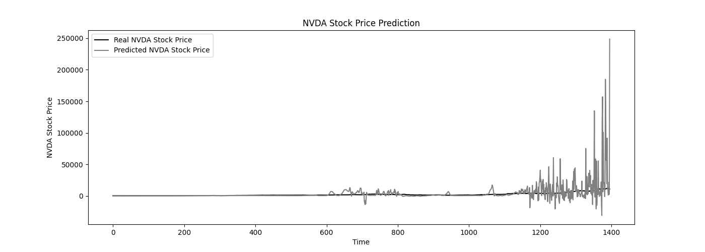
Step 6: Visualizing the Results

Finally, we visualize the predicted stock prices against the actual stock prices to assess the model’s performance.

import matplotlib.pyplot as plt

plt.figure(figsize=(14,5))
plt.plot(y_test, color='black', label='Real NVDA Stock Price')
plt.plot(y_pred, color='gray', label='Predicted NVDA Stock Price')
plt.title('NVDA Stock Price Prediction')
plt.xlabel('Time')
plt.ylabel('NVDA Stock Price')
plt.legend()
plt.show()

The following plot shows the predicted Nvidia stock prices (gray line) against the actual stock prices (black line), demonstrating the model’s accuracy.

Conclusion

Building an RNN with LSTM layers for stock prediction involves several steps, from preparing the data and building the model to training and making predictions. LSTM networks are particularly effective for this type of time-series forecasting due to their ability to capture long-term dependencies in the data. By following the steps outlined above, you can build and evaluate your own stock price prediction model.

This approach can be adapted and extended for other types of sequential data and prediction tasks, making it a versatile tool in your machine learning toolkit.