Skip to content

2023

Understanding AdaBoost and Gradient Boosting Machine

In the realm of machine learning, two of the most potent and widely-used algorithms are AdaBoost and Gradient Boosting Machine (GBM). Both of these techniques are used for boosting, a method that sequentially applies weak learners to improve model accuracy. Let's delve deeper into each of these algorithms, their workings, and differences.

AdaBoost: The Adaptive Boosting Pioneer

AdaBoost, short for Adaptive Boosting, was introduced in the late 1990s. This algorithm has a unique approach to improving model accuracy by focusing on the mistakes of previous iterations.

How AdaBoost Works

  1. Initial Equal Weighting: AdaBoost starts by assigning equal weights to all data points in the training set.
  2. Sequential Learning: It then applies a weak learner (like a decision tree) to classify the data.
  3. Emphasis on Errors: After each round, AdaBoost increases the weights of incorrectly classified instances. This makes the algorithm focus more on the difficult cases in subsequent iterations.
  4. Combining Learners: The final model is a weighted sum of the weak learners, with more accurate learners given higher weights.

AdaBoost's Key Features

  • Simplicity and Flexibility: It can be used with any learning algorithm and is easy to implement.
  • Sensitivity to Noisy Data: AdaBoost can be sensitive to outliers since it focuses on correcting mistakes.

Gradient Boosting Machine: The Evolution

Gradient Boosting Machine (GBM) is a more general approach and can be seen as an extension of AdaBoost. It was developed to address some of AdaBoost's limitations, particularly in handling a broader range of loss functions.

How GBM Works

  1. Sequential Learning with Gradient Descent: GBM uses gradient descent to minimize errors. It builds one tree at a time, where each new tree helps to correct errors made by the previous ones.
  2. Handling Various Loss Functions: Unlike AdaBoost, which focuses on classification errors, GBM can optimize any differentiable loss function, making it more versatile.
  3. Control Over Fitting: GBM includes parameters like the number of trees, tree depth, and learning rate, providing better control over fitting.

GBM's Key Features

  • Flexibility: It can be used for both regression and classification tasks.
  • Better Performance: Often provides better predictive accuracy than AdaBoost.
  • Complexity and Speed: More complex and typically slower to train than AdaBoost, especially with large datasets.

AdaBoost vs Gradient Boosting Machine: A Comparison

While both algorithms are based on the idea of boosting, they differ significantly in their approach and capabilities:

  • Focus: AdaBoost focuses on classification errors, while GBM focuses on minimizing a loss function.
  • Flexibility: GBM is more flexible than AdaBoost in terms of handling different types of data and loss functions.
  • Performance: GBM generally provides better performance, especially on more complex datasets.
  • Ease of Use: AdaBoost is simpler and faster to train, making it a good starting point for beginners.

Conclusion

Both AdaBoost and Gradient Boosting Machine have their unique strengths and are powerful tools in the machine learning toolbox. The choice between them depends on the specific requirements of the task, the nature of the data, and the desired balance between accuracy and computational efficiency. As machine learning continues to evolve, these algorithms will undoubtedly remain fundamental, continuing to empower new and innovative applications.


Understanding AdaBoost and Gradient Boosting Machine

Hello and welcome to "Continuous Improvement," the podcast where we explore the fascinating world of machine learning and its impact on technology and our lives. I'm your host, Victor, and today, we're diving into the realm of two potent algorithms: AdaBoost and Gradient Boosting Machine, or GBM. These techniques are crucial in the world of boosting, a method enhancing model accuracy by applying a series of weak learners. So, let's get started!

First up, let's talk about AdaBoost, the Adaptive Boosting Pioneer, introduced in the late 1990s. AdaBoost has a unique approach to improving model accuracy, focusing on the mistakes of previous iterations. Here’s how it works:

  1. Initial Equal Weighting: AdaBoost begins by assigning equal weights to all data points in the training set.
  2. Sequential Learning: It then applies a weak learner, like a decision tree, to classify the data.
  3. Emphasis on Errors: After each round, AdaBoost increases the weights of incorrectly classified instances, focusing more on difficult cases in subsequent iterations.
  4. Combining Learners: The final model is a weighted sum of these weak learners, with more accurate ones given higher weights.

AdaBoost is known for its simplicity and flexibility, making it a popular choice. However, it's also sensitive to noisy data, which can be a downside.

Moving on, let's discuss Gradient Boosting Machine, or GBM. GBM is a more general approach and can be seen as an extension of AdaBoost, developed to address some of its limitations, especially in handling a broader range of loss functions.

Here's how GBM operates:

  1. Sequential Learning with Gradient Descent: GBM uses gradient descent to minimize errors. It builds one tree at a time, each new tree correcting errors made by the previous ones.
  2. Handling Various Loss Functions: Unlike AdaBoost, GBM can optimize differentiable loss functions, making it more versatile.
  3. Control Over Fitting: With parameters like the number of trees, tree depth, and learning rate, GBM offers better control over fitting.

GBM is flexible, often providing better predictive accuracy than AdaBoost. However, it's more complex and typically slower to train, particularly with large datasets.

Now, let's compare AdaBoost and Gradient Boosting Machine. While both are based on boosting, their approaches and capabilities differ significantly.

  • Focus: AdaBoost centers on classification errors, while GBM aims to minimize a loss function.
  • Flexibility: GBM handles different types of data and loss functions more flexibly than AdaBoost.
  • Performance: Generally, GBM offers better performance, especially on complex datasets.
  • Ease of Use: AdaBoost is simpler and faster to train, making it ideal for beginners.

In conclusion, both AdaBoost and Gradient Boosting Machine have unique strengths, making them powerful tools in machine learning. The choice between them depends on your task's specific requirements, the data's nature, and the balance you seek between accuracy and computational efficiency. As machine learning continues to evolve, these algorithms will undoubtedly remain fundamental, empowering innovative applications.

That's all for today's episode of "Continuous Improvement." I hope you found our journey through AdaBoost and GBM insightful. Don't forget to subscribe for more episodes on machine learning and technology. I'm Victor, and until next time, keep learning and keep improving!

理解AdaBoost和梯度提升機器

在機器學習領域中,兩種最有力且被廣泛使用的算法是AdaBoost和梯度提升機器(GBM)。這兩種技術都被用於提升,一種逐步應用弱學習器以提高模型準確性的方法。讓我們深入了解每種算法的工作原理,以及它們的區別。

AdaBoost: 自我調整增強的先驅

AdaBoost,全名為自適應增強,於20世紀90年代末被介紹。這個算法通過專注於前一個迭代的錯誤來改進模型的準確性有一種獨特的方法。

AdaBoost的工作原理

  1. 初始等權重:AdaBoost首先給訓練集中的所有數據點分配相同的權重。
  2. 序列學習:然後,它應用一個弱學習器(如決策樹)對數據進行分類。
  3. 對錯誤的強調:每一輪過後,AdaBoost會增加分類不正確的實例的權重。這使得算法在後續的迭代中更加專注於困難的案例。
  4. 組合學習器:最終的模型是弱學習器的加權和,其中更準確的學習器給予更高的權重。

AdaBoost的主要特點

  • 簡單和靈活:它可以與任何學習算法一起使用,並且易於實現。
  • 對噪聲數據的敏感性:AdaBoost可能對異常值敏感,因為它專注於糾正錯誤。

梯度增強機:演進

梯度提升機(GBM)是一種更一般的方法,可以被視為AdaBoost的擴充。它被開發出來解決AdaBoost的一些限制,尤其是在處理更廣泛的損失函數方面。

GBM的工作原理

  1. 用梯度下降進行序列學習:GBM使用梯度下降來最小化錯誤。它一次構建一棵樹,每棵新樹都有助於糾正前一棵樹的錯誤。
  2. 處理各種損失函數:與AdaBoost不同,調用對分類誤差,GBM可以優化任何可微分的損失函數,使其更具通用性。
  3. 對擬合的控制:GBM包含樹的數量,樹的深度和學習率等參數,提供了更好的對擬合的控制。

GBM的主要特點

  • 靈活性:它可以用於回歸和分類任務。
  • 更好的性能:通常比AdaBoost提供更好的預測準確性。
  • 複雜性和速度:比AdaBoost更複雜,尤其是對於大數據集來說,訓練通常較慢。

AdaBoost vs 梯度提升機:比較

雖然這兩種算法都基於增強的想法,但在其方法和能力方面有顯著的區別:

  • 焦點:AdaBoost關注分類錯誤,而GBM關注最小化損失函數。
  • 靈活性:在處理不同類型的數據和損失函數方面,GBM比AdaBoost更靈活。
  • 性能:GBM通常提供更好的性能,尤其是對於更複雜的數據集。
  • 使用的簡便性:AdaBoost更簡單,更快地訓練,因此它是初學者的一個好的起點。

結論

Adaboost和梯度提升機都有自己獨特的優點,並且是機器學習工具箱中的強大工具。在它們之間的選擇取決於任務的具體要求,數據的性質,以及在準確度和計算效率之間的平衡。隨著機器學習的不斷發展,這些算法無疑將繼續存在,並繼續賦予新的和創新的應用。

Understanding Bootstrap Aggregation and Random Forest

In the world of machine learning, there are numerous techniques and algorithms that empower predictive modeling and data analysis. Two such powerful methods are Bootstrap Aggregation, commonly known as Bagging, and Random Forest. These techniques are widely used for their robustness and ability to improve the accuracy and stability of machine learning models.

What is Bootstrap Aggregation (Bagging)?

Bootstrap Aggregation, or Bagging, is an ensemble learning technique used to improve the stability and accuracy of machine learning algorithms. It reduces variance and helps to avoid overfitting. The concept of Bagging was introduced by Leo Breiman in 1994 and has since become a cornerstone in the field of machine learning.

How Does Bagging Work?

Bagging involves creating multiple versions of a predictor and using these to get an aggregated predictor. The main steps are:

  1. Random Sampling with Replacement: The original dataset is sampled randomly with replacement, creating multiple bootstrapped datasets.
  2. Model Training: A model is trained separately on each bootstrapped dataset.
  3. Aggregation of Predictions: The predictions from each model are combined (usually by averaging for regression problems or voting for classification problems) to form a final prediction.

The beauty of Bagging lies in its simplicity and effectiveness, especially for decision tree algorithms, where it significantly reduces variance without increasing bias.

Random Forest: An Extension of Bagging

Random Forest is a popular ensemble learning technique that builds upon the concept of Bagging. Developed also by Leo Breiman, it involves constructing a multitude of decision trees at training time and outputting the class that is the mode of the classes (classification) or mean prediction (regression) of the individual trees.

How Does Random Forest Differ from Basic Bagging?

  1. Use of Decision Trees: Random Forest specifically uses decision trees as its base learners.
  2. Feature Randomness: When building each tree, a random subset of features is chosen. This ensures that the trees are de-correlated and makes the model more robust to noise.
  3. Multiple Trees: A Random Forest typically involves a larger number of trees, providing a more accurate and stable prediction.

Advantages of Random Forest

  • High Accuracy: Random Forests often produce highly accurate models, especially for complex datasets.
  • Robust to Overfitting: Due to the averaging of multiple trees, the risk of overfitting is lower compared to individual decision trees.
  • Handles Large Datasets Efficiently: They are capable of handling large datasets with higher dimensionality.

Applications and Considerations

Both Bagging and Random Forest find applications in various fields, including finance for credit scoring, biology for gene classification, and many areas of research and development. However, while using these techniques, one must be mindful of the following:

  • Computational Complexity: Both methods can be computationally intensive, especially Random Forest with a large number of trees.
  • Interpretability: Decision trees are inherently interpretable, but when combined into a Random Forest, the interpretability decreases.
  • Parameter Tuning: Tuning parameters like the number of trees, depth of trees, and number of features considered at each split is crucial for optimal performance.

Conclusion

Bootstrap Aggregation and Random Forest are powerful techniques in the arsenal of a data scientist. By understanding and correctly applying these methods, one can significantly improve the performance of machine learning models, tackling both bias and variance, and thereby making robust and accurate predictions. As with any tool, their effectiveness depends largely on the skill and understanding of the practitioner in applying them to the right kind of problems.

Understanding Bootstrap Aggregation and Random Forest

Hello, and welcome back to "Continuous Improvement," the podcast where we dive deep into the ever-evolving world of technology and data science. I’m your host, Victor, and today, we're unpacking two powerful tools in the machine learning toolbox: Bootstrap Aggregation, or Bagging, and Random Forest. So, let's get started!

First up, let's talk about Bootstrap Aggregation, commonly known as Bagging. Developed by Leo Breiman in 1994, this ensemble learning technique is a game-changer in reducing variance and avoiding overfitting in predictive models. But what exactly is it, and how does it work?

Bagging involves creating multiple versions of a predictor, each trained on a bootstrapped dataset - that's a fancy way of saying a dataset sampled randomly with replacement from the original set. These individual models then come together, their predictions combined through averaging or voting, to form a more accurate and stable final prediction. It’s particularly effective with decision tree algorithms, where it significantly reduces variance without upping the bias.

Moving on to Random Forest, a technique that builds upon the concept of Bagging. Also pioneered by Breiman, Random Forest stands out by specifically using decision trees as base learners and introducing feature randomness. It creates a forest of decision trees, each trained on a random subset of features, and then aggregates their predictions. This not only enhances the model's accuracy but also makes it robust against overfitting and noise.

Now, why should we care about Random Forest? It's simple: high accuracy, especially for complex datasets, resistance to overfitting, and efficient handling of large datasets with many features. That's a powerful trio, right?

Both Bagging and Random Forest are not just theoretical marvels. They have practical applications in fields like finance for credit scoring, biology for gene classification, and various areas of research and development. However, it's important to be aware of their complexities. They can be computationally intensive, especially with a large number of trees in Random Forest, and their interpretability can decrease compared to individual decision trees.

In conclusion, Bootstrap Aggregation and Random Forest are invaluable for any data scientist. They tackle bias and variance, leading to robust and accurate predictions. Remember, their effectiveness largely depends on how well they are applied to the right problems.

That's all for today’s episode of "Continuous Improvement." I hope you found our journey through Bagging and Random Forest insightful. Stay tuned for our next episode, where we'll explore more exciting advancements in machine learning. This is Victor, signing off. Keep learning, keep improving!

理解Bootstrap Aggregation與隨機森林

在機器學習的世界中,有許多技術和算法可以強化預測模型和數據分析。其中兩種強大的方法就是Bootstrap Aggregation,通常被稱為Bagging,以及隨機森林。這兩種技術因其穩健性以及能夠提高機器學習模型的精確性和穩定性而被廣泛使用。

什麼是Bootstrap Aggregation (Bagging)?

Bootstrap Aggregation,即Bagging,是一種集成學習技術,用於提高機器學習算法的穩定性和準確性。它能減少方差並有助於避免過度擬合。Bagging的概念由Leo Breiman於1994年提出,並已成為機器學習領域的基石。

Bagging如何運作?

Bagging包括創建預測器的多個版本並使用它們來得到一個聚合的預測器。主要步驟包括:

  1. 隨機抽樣並替換:原始資料集經過隨機抽樣並替換,創造出多個自助的資料集。
  2. 模型訓練:每個自助的資料集都單獨訓練一個模型。
  3. 預測結果匯總:所有模型的預測結果合併(通常對於迴歸問題進行平均或對於分類問題進行投票)形成最終的預測。

Bagging的美在於其簡單有效,特別是對於決策樹算法,它顯著地降低了方差而沒有增加偏差。

隨機森林:Bagging的擴展

隨機森林是一種流行的集成學習技術,建立在Bagging的概念之上。由Leo Breiman同樣發展出來,它包括在訓練時構建多個決策樹,並輸出各決策樹的類別模式(分類)或平均預測(迴歸)。

隨機森林與基礎Bagging的區別?

  1. 使用決策樹:隨機森林具體使用決策樹作為其基礎學習器。
  2. 特徵隨機選擇:構建每棵樹時,會選擇一組隨機的特徵子集。這確保了樹的相關性降低,並使模型對噪音更具韌性。
  3. 多棵樹:隨機森林通常包括更多的樹,提供更準確和穩定的預測。

隨機森林的優點

  • 高精確度:對於複雜的數據集,隨機森林常能產生高精確度的模型。
  • 對於過度擬合的韌性:由於多個樹的平均,相較於單一的決策樹,隨機森林對於過度擬合的風險降低。
  • 有效處理大數據集:它們能夠有效地處理具有較高維度的大數據集。

應用與考量

Bagging和隨機森林在許多領域都有應用,包括金融中的信用評分,生物學中的基因分類,以及各種研究和開發領域。然而,在使用這些技術時,必須謹記以下幾點:

  • 計算複雜性:這兩種方法可能會非常消耗計算資源,特別是隨機森林中樹的數量較多的情況。
  • 可解釋性:決策樹本質上是可以解釋的,但當它組合成隨機森林時,可解釋性會降低。
  • 參數調整:調整像樹的數量、樹的深度以及每個分割點考慮的特徵數量等參數對於獲得最佳性能非常關鍵。

結論

在數據科學家的工具箱中,Bootstrap Aggregation和隨機森林都是強大的技術。通過理解和正确應用這些方法,可以顯著提高機器學習模型的性能,同時處理偏差和方差,從而使預測更為穩健和準確。像任何工具一樣,他們的有效性大部分取決於應用他們來解決適當問題的實踐者的技能和理解。

Understanding Inertia and Silhouette Coefficient - Key Metrics in Clustering Analysis

Clustering is a fundamental technique in data science and machine learning, used for grouping similar data points together. Among the various metrics to evaluate the quality of clustering, Inertia and Silhouette Coefficient stand out for their insightful feedback on cluster quality. Let's dive into what these metrics are and how they help in analyzing clusters.

What is Inertia?

Inertia, also known as within-cluster sum-of-squares, measures the compactness of clusters. It calculates the total variance within the clusters. In simpler terms, it's the sum of the distances of each data point in a cluster to the centroid of that cluster, squared and summed up for all clusters.

Key Points:

  • A lower inertia value implies a better model, as it indicates tighter clustering.
  • However, the inertia metric has a drawback: it keeps decreasing with an increase in the number of clusters ( k ). This is where the "elbow method" is often used to find the optimal ( k ).
Understanding the Silhouette Coefficient

The Silhouette Coefficient is a measure of how similar an object is to its own cluster (cohesion) compared to other clusters (separation). The silhouette ranges from -1 to +1, where a high value indicates that the object is well matched to its own cluster and poorly matched to neighboring clusters.

Key Points:

  • A high silhouette score indicates well-clustered data.
  • Unlike inertia, the silhouette score provides more nuanced insight into the separation distance between the resulting clusters.
When to Use Each Metric
  1. Inertia:

  2. Good for assessing the compactness of clusters.

  3. Best when used with the elbow method to determine the optimal number of clusters.
  4. More sensitive to the scale of the data, so normalization or standardization might be necessary.

  5. Silhouette Coefficient:

  6. Ideal for validating the consistency within clusters of data.
  7. Useful when the number of clusters is not known.
  8. Offers a more balanced view, incorporating both cohesion and separation.
Conclusion

Inertia and Silhouette Coefficient are crucial metrics for evaluating the performance of clustering algorithms like K-Means. They provide different perspectives: inertia focuses on internal cluster compactness, while silhouette coefficient assesses how well-separated the clusters are. The choice of metric often depends on the specific requirements of the clustering problem at hand.

Understanding Inertia and Silhouette Coefficient - Key Metrics in Clustering Analysis

Welcome back to the "Continuous Improvement" podcast, where we delve into the intriguing world of data science and machine learning. I'm your host, Victor, and today we're going to unpack a critical aspect of clustering techniques - evaluating cluster quality. So, let's get right into it.

First off, what is clustering? It's a cornerstone in data science, essential for grouping similar data points together. And when we talk about evaluating these clusters, two metrics really stand out: Inertia and Silhouette Coefficient. Understanding these can significantly enhance how we analyze and interpret clustering results.

Let's start with Inertia. Also known as within-cluster sum-of-squares, this metric is all about measuring how tight our clusters are. Imagine this: you're looking at a cluster and calculating how far each data point is from the centroid of that cluster. Sum up these distances, square them, and that's your inertia. A lower value? That's what we're aiming for, as it indicates a snug, compact cluster.

But, and there's always a but, inertia decreases as we increase the number of clusters. This is where the elbow method comes into play, helping us find the sweet spot for the number of clusters.

Moving on to the Silhouette Coefficient. This one's a bit more nuanced. It's like asking each data point, "How well do you fit in your cluster, and how badly do you fit in neighboring clusters?" With values ranging from -1 to +1, a high score means the data is well-clustered.

Unlike inertia, the Silhouette Coefficient doesn't just focus on the tightness of the cluster but also how distinct it is from others.

So, when do we use each metric? Inertia is your go-to for checking cluster compactness, especially with the elbow method. But remember, it's sensitive to the scale of data. On the other hand, the Silhouette Coefficient is perfect for validating consistency within clusters, particularly when you're not sure about the number of clusters to start with.

In conclusion, both Inertia and Silhouette Coefficient are pivotal in the realm of clustering algorithms like K-Means. They offer different lenses to view our data - inertia looks inward at cluster compactness, while the silhouette coefficient gazes outward, assessing separation between clusters.

That's it for today's episode on "Continuous Improvement." I hope you found these insights into Inertia and Silhouette Coefficient as fascinating as I do. Join us next time as we continue to explore the ever-evolving world of data science. Until then, keep analyzing and keep improving!

理解慣性和輪廓係數 - 分群分析中的關鍵指標

分群是資料科學和機器學習中的基本技術,用於將相似的資料點分組在一起。在評估分群質量的各種指標中,慣性輪廓係數以其對分群質量深入的反饋而脫穎而出。讓我們深入了解這些指標是什麽,以及它們如何幫助分析分群。

什麽是慣性?

慣性也稱為群內平方和,用於衡量分群的緊密度。它計算分群內的總變異。簡單來說,就是每個資料點到該分群重心的距離的平方值的總和,並為所有分群加總。

關鍵點:

  • 較低的慣性值表示模型較好,因為它表示分群較為緊密。
  • 但是,慣性指標有一個缺點:隨著分群數量(k)的增加,它會持續下降。這就是常常使用"肘部方法"來找到最佳的(k)的地方。
理解輪廓係數

輪廓係數是一種衡量物體與自己分群的相似度(凝聚力)與其他分群(分離度)之間的差異的度量。輪廓值範圍是-1到+1,其中高值表明物體與自己的分群匹配得很好,並且與相鄰分群的匹配度差。

關鍵點:

  • 高輪廓得分表示資料分群良好。
  • 與慣性不同,輪廓得分對分群間的分離距離提供了更細微的見解。
何時使用每一個指標
  1. 慣性

  2. 良好的分群緊密度評估工具。

  3. 目測分群最佳數量時與肘部方法配合使用最佳。
  4. 對資料的尺度更敏感,因此可能需要正規化或標準化。

  5. 輪廓係數

  6. 驗證分群資料內部一致性的理想工具。
  7. 在不知道分群數量的情況下很有用。
  8. 提供了更均衡的視角,包括凝聚力和分離度。
結論

慣性和輪廓係數是評估像K-Means這樣的分群演算法性能的關鍵指標。它們提供了不同的視角:慣性專注於內部分群的緊密度,而輪廓係數評估分群之間的分離性如何。選擇使用哪個指標通常取決於手頭分群問題的具體要求。

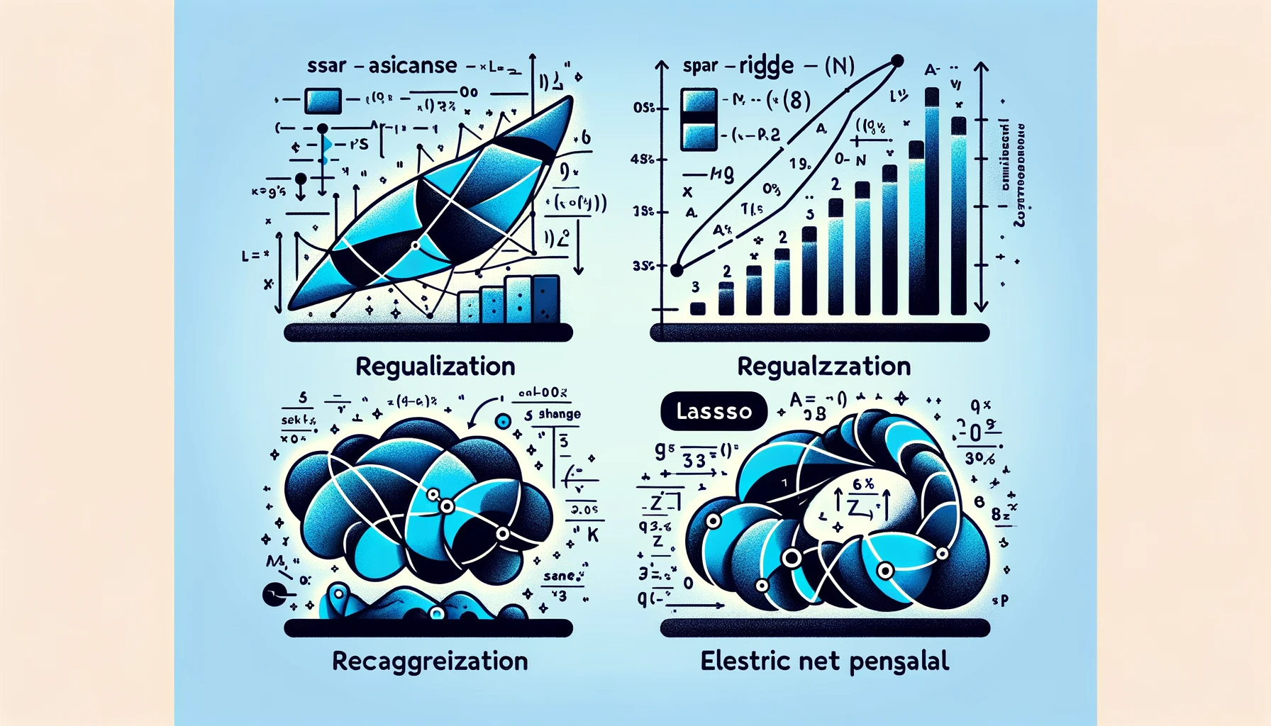
Understanding Regularization - Lasso, Ridge, and Elastic Net Regression

In the field of machine learning and statistical modeling, regularization is a crucial technique used to prevent overfitting and improve the generalization of models. This blog post will delve into three popular regularization methods: Lasso, Ridge, and Elastic Net Regression, elucidating how they function and when to use them.

What is Regularization?

Regularization is a technique used to reduce overfitting in machine learning models. Overfitting occurs when a model learns not only the underlying pattern in the training data but also the noise. This leads to poor performance on unseen data. Regularization addresses this issue by adding a penalty term to the loss function used to train the model. This penalty term constrains the model, making it simpler and less prone to overfitting.

Ridge Regression (L2 Regularization)

Ridge Regression, also known as L2 regularization, adds a penalty equal to the square of the magnitude of the coefficients. The regularization term is added to the loss function, and it includes a tuning parameter, λ (lambda), which determines the strength of the penalty. A higher value of λ shrinks the coefficients more, leading to a simpler model.

Key Features of Ridge Regression:

  • It tends to shrink the coefficients of the model uniformly.
  • Suitable for scenarios where many features have a small or moderate effect on the output variable.
  • Ridge regression does not perform variable selection - it includes all features in the final model.

Lasso Regression (L1 Regularization)

Lasso Regression, short for Least Absolute Shrinkage and Selection Operator, involves L1 regularization. It adds a penalty equal to the absolute value of the magnitude of coefficients. Like Ridge, it also has a tuning parameter, λ, which controls the strength of the penalty.

Key Features of Lasso Regression:

  • Lasso can shrink the coefficients of less important features to exactly zero, thus performing variable selection.
  • Useful when we have a large number of features, and we suspect that many of them might be irrelevant or redundant.
  • Can lead to sparse models where only a subset of the features contributes to the prediction.

Elastic Net Regression

Elastic Net Regression is a hybrid approach that combines both L1 and L2 regularization. It adds both penalties to the loss function. Elastic Net is particularly useful when there are multiple correlated features. It includes two parameters: λ (like in Lasso and Ridge) and α, which balances the weight given to L1 and L2 regularization.

Key Features of Elastic Net Regression:

  • Balances the properties of both Lasso and Ridge.
  • Works well when several features are correlated.
  • Elastic Net can be tuned to behave like Lasso or Ridge regression by adjusting the α parameter.

Choosing the Right Regularization Method

The choice between Lasso, Ridge, and Elastic Net depends on the data and the problem at hand:

  • Ridge is a good default when there is not much feature selection needed or if the features are expected to have roughly equal importance.
  • Lasso is preferred if feature selection is essential, and there is a need to identify the most significant variables.
  • Elastic Net is ideal when there are multiple correlated features, or a balance between feature selection and uniform coefficient reduction is required.

Conclusion

Regularization is a powerful tool in machine learning, helping to enhance the performance and interpretability of models. Lasso, Ridge, and Elastic Net are versatile methods that can be applied to various regression problems. Understanding their differences and applications is key to building robust and accurate predictive models.